Higher-Dimensional Sledgehammers and Exponentially-Growing Disincentives
Written April 17, 2020.
Abstract
In this article, we first generalize the Sledgehammer-based commutator [[R’, F], D] as a way to solve \(n\)-dimensional \(s^n\) Rubik’s cubes (where \(s \ge 2, n \ge 3\)). We then analyze the commutator movecount with respect to \(s\) and \(n\), and derive asymptotic bounds for the expected solution length of an \(s^n\) Rubik’s cube. We consider two different solving approaches: one where we use generalized commutators for every piece type, and one where we use a modification of Roice’s method with reduction without freeslicing. We find that the growth rate of the solution length is exponential in both cases, greatly disincentivizing solving past three dimensions using these approaches without macros.
TL;DR: See the conclusion for a summary of our findings.
Sledgehammers
The [R’, F] commutator is known as the Sledgehammer in speedcubing parlance. We can use the Sledgehammer-based [[R’, F], D] to solve the corners (Figure 1), and the Sledgehammer-based [[R’, F], E] to solve the edges.
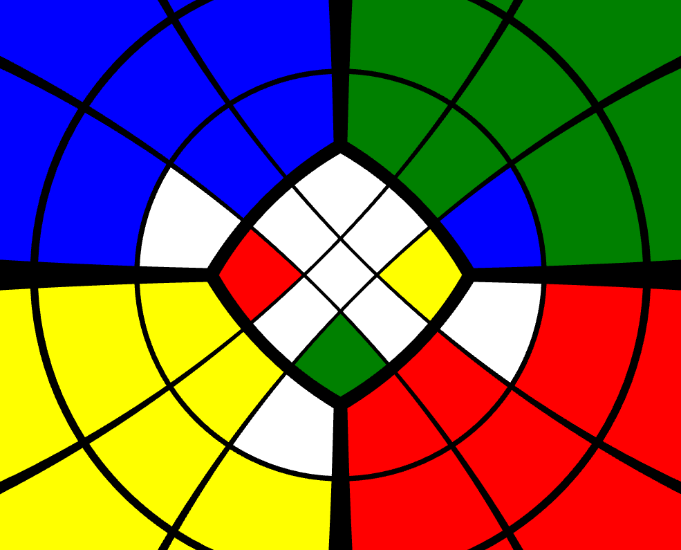
Figure 1: [[R’, F], D] performed on a 3x3x3, where the U face is green and the F face is white.
We can apply these Sledgehammer-based commutators to higher-order three-dimensional \(s^3\) Rubik’s cubes by generalizing the commutator to [[Jr’, F], Kd], where \(J\) and \(K\) refer to some slice depth, \(1 \le J, K \le \lceil s/2 \rceil\). By varying \(J\) and \(K\), we induce three-cycles on different sets of pieces.
When we apply this approach to higher dimensions, the commutator generalizes to \([[[[S, D_3], D_4], \ldots], D_n]\), where the effect of \(S\) is equivalent to that of the Sledgehammer, and \(D_m\) is some equivalent to the D move on a 3x3x3 for \(3 \le m \le n\). In essence, each additional \(D_m\) causes the commutator to selectively cycle a smaller number of pieces, until only three are cycled.
For example, in four dimensions, we can do [[[TF, RF’], DF], [LU: 3TU]] to cycle three 4-coloured pieces on a \(3^4\) Rubik’s cube (Figure 2), and generalize to [[[TF, RF’], 1/2DF], [LU: 2/3TU]] in order to cycle other piece types on the \(3^4\) Rubik’s cube, where 1/2 in this case means to turn either the first or second layer, and 2/3 in this case means to turn either the second or third layer. We can use similar logic to solve any \(s^4\) Rubik’s cube, where \(s \ge 2\).
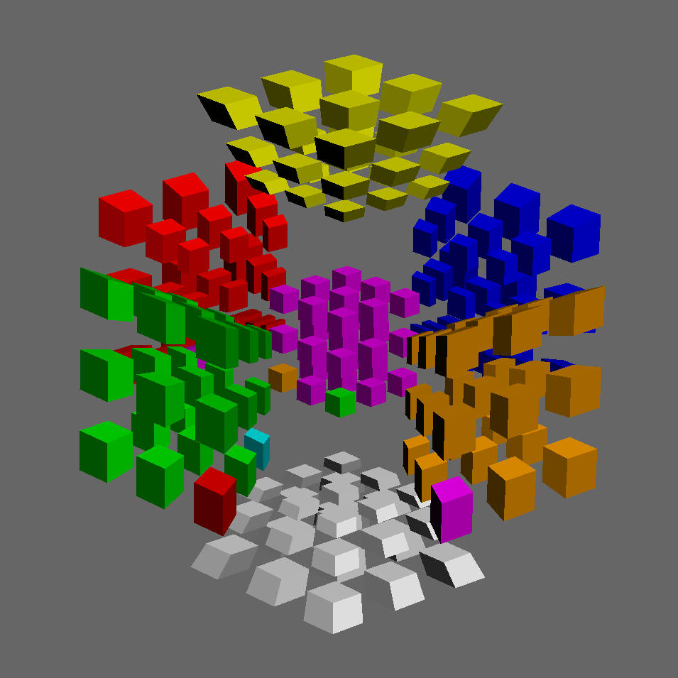
Figure 2: [[[TF, RF’], DF], [LU: 3TU]] performed on a 3x3x3x3.
However, every time we go up a dimension, we nest the commutator another layer deep, and the length of the commutator at least doubles in size. Thus, the commutator length grows at a rate of \(\Omega(2^n)\), where \(n\) is the dimension number.
Bounding the Solution Lengths
We now estimate asymptotic bounds for the expected solution lengths required to solve the \(s^n\) Rubik’s cube, assuming \(s \ge 2\) is fixed, and \(n \ge 3\). These bounds do not give exact solution movecount numbers, but allow us to see the overall trend in expected solution lengths as \(n\) increases.
We firstly assume that the puzzle is well-scrambled, meaning that all pieces are permuted incorrectly relative to their solved positions. In reality, there are often pieces that are permuted correctly, but we assume that:
- There are not enough pieces that are both correctly oriented and permuted to significantly affect the estimate.
- Pieces that are permuted correctly but oriented incorrectly require up to twice as much effort to solve as pieces that are permuted incorrectly. This constant factor is then discarded when using big-\(O\) notation and its variants.
We then assume each commutator only solves a single piece. In three dimensions, it is easy to perform setup moves to place two pieces at a time with these commutators. However, the number of possible orientations an \(m\)-coloured piece can have is bounded by \(\Theta(m!)\), so it takes much longer to correctly orient and set up pieces in higher dimensions.
We also do not count setup moves, because the number of setup moves required to solve the puzzle varies depending on the given cycle and the commutators used. A rough estimate for the number of moves required to solve an \(s^n\) Rubik’s cube, including setup moves, can be made by doubling the initial left-hand-side expressions given in the equations below.
Lastly, we do not take the fact that odd-length \(s^n\) Rubik’s cubes have fixed centers into consideration when doing the calculations, which overestimates the number of centers that need to be solved for these puzzles by \(2n\) (out of \(2n(s-2)^{n-1}\) centers in total). We assume this overestimation is negligible, because the total number of pieces grows exponentially as \(n\) increases, whereas \(2n\) grows linearly.
Solving using Pure Commutators
Firstly, we consider an approach where the solver uses pure commutators for the entire solve, meaning that \(m\)-coloured pieces are solved using commutators that only swap around \(m\)-coloured pieces. For this case, every commutator is of the form \([[[[S, D_3], D_4], \ldots], D_n]\), and so it takes \(\Omega(2^n)\) moves to solve each \(m\)-coloured piece for all \(1 \le m \le n\).
Theorem 1.1: Assume \(s \ge 3\) is fixed, and let \(n \ge 3\). A bound for the expected solution length for the \(s^n\) Rubik’s cube using pure commutators is \(\Omega((2s)^n)\) moves.
Proof: For each \(m\)-coloured piece, we expect to use \(\Omega(2^n)\) moves. By Theorem 3.2 in [1], there are \(2^m {n \choose m} (s - 2)^{n - m}\) \(m\)-coloured pieces in an \(s^n\) Rubik’s cube. Therefore, we obtain the following bound:
\[\begin{align*} \sum_{m = 1}^n \Omega(2^n) 2^m {n \choose m} (s - 2)^{n - m} &= \Omega(2^n) (s - 2)^n \sum_{m = 1}^n \left({2 \over s - 2}\right)^m {n \choose m} \\ &= \Omega(2^n) (s - 2)^n \left[\left({2 \over s - 2} + 1\right)^n - 1\right] \\ &= \Omega(2^n) (s - 2)^n \left[\left({s \over s - 2}\right)^n - 1\right] \\ &= \Omega(2^n)(s^n - (s - 2)^n) \\ &= \Omega(2^n) \Theta(s^n) = \Omega((2s)^n) \end{align*}\]as desired. \(\square\)
For example, the expected number of moves to solve the \(3^n\) Rubik’s cube is bounded by \(\Omega(6^n)\).
We cannot use the equations above for \(s = 2\), because that ends up dividing by zero. However, we can easily run a separate set of calculations for that case.
Theorem 1.2: Let \(n \ge 3\). A bound for the expected solution length for the \(2^n\) Rubik’s cube using pure commutators is \(\Omega(4^n)\) moves.
Proof: The \(2^n\) Rubik’s cube has \(2^n\) \(n\)-coloured pieces, by Corollary 3.3 in [1]. For each piece, we expect to take \(\Omega(2^n)\) moves, so the expected solution length for the \(2^n\) Rubik’s cube is bounded by \(\Omega(2^n)2^n = \Omega(4^n)\). \(\square\)
Solving using Reduction and Roice’s Method
For the \(3^n\) Rubik’s cube in particular, we can consider using a variation of Roice’s Method, which is a higher-dimensional generalization of Marshall’s Ultimate Solution.
In this case, we solve the pieces in order from 1-coloured pieces to \(n\)-coloured pieces. In other words, while solving \(m\)-coloured pieces, we can alter any \(p\)-coloured piece where \(m + 1 \le p \le n\). Due to this additional freedom, we can use commutators of the form \([[[[S, D_3], D_4], \ldots], D_m]\) to solve \(m\)-coloured pieces, and thus use \(\Omega(2^m)\) moves to solve each \(m\)-coloured piece.
Note that this optimization does not change anything for the \(2^n\) Rubik’s cube—we are still stuck with \(2^n\) \(n\)-coloured pieces, and thus still obtain the bound of \(\Omega(4^n)\) from Theorem 1.2.
Theorem 2.1: A bound for the expected solution length for the \(3^n\) Rubik’s cube using Roice’s Method is \(\Omega(5^n)\) moves.
Proof: We have a bound of \(\Omega(2^m)\) moves per \(m\)-coloured piece. Combining this information with Corollary 3.4 in [1], we obtain the following bound:
\[\begin{align*} \sum_{m = 1}^n \Omega(2^m) 2^m {n \choose m} &= \Omega\left(\sum_{m = 1}^n 4^m {n \choose m}\right) \\ &= \Omega\left((4 + 1)^n - 1\right) \\ &= \Omega(5^n) \end{align*}\]as desired. \(\square\)
Note that it is not possible to directly solve an \(s^n\) Rubik’s cube using Roice’s method for \(s \ge 4\). For example, if we have a 3-coloured wing piece placed correctly on a \(4^4\) Rubik’s cube, then we must use a pure commutator to place its adjacent wing piece. Using just \([S, D_3]\) will place this second wing piece successfully, but it will simultaneously kick out the first one.
However, we can first reduce the puzzle to a \(3^n\) Rubik’s cube, and then solve the resulting \(3^n\) Rubik’s cube in \(\Omega(5^n)\) moves by Theorem 2.1. We assume the additional movecount required to resolve parity errors is negligible.
While forming blocks (the higher-dimensional equivalent of pairs), we eventually have to use commutators of the form \([[[[S, D_3], D_4], \ldots], D_n]\), or \(n\)-dimensional RKT sequences, to pair up the last few pieces. In both cases, this results in \(\Omega(2^n)\) moves spent per pairing. However, a vast majority of the pairings, assuming we pair the 1-coloured pieces first, then the 2-coloured pieces, and so on, can be done in \(\Omega(2^m)\) moves, where \(m\) is the number of colours on the piece. Thus, we assume \(\Omega(2^m)\) moves are spent per \(m\)-coloured piece pairing.
Lemma 2.2: Fix \(s \ge 1\), and let \(n \ge 1\). Assume we form a block of size \(s^n\) as follows:
We find \(s\) blocks of size \(1\), and then join them together to form a block of size \(s\). Then, for \(1 \le m \le n-1\), we form \(s-1\) more blocks of size \(s^m\), and then join the \(s\) blocks of size \(s^m\) together to form a block of size \(s^{m+1}\). We end up with a block of size \(s^n\).
Using this approach, we claim there are \(s^n - 1\) pairings required to form a block of size \(s^n\).
Proof: We use induction on \(n \ge 1\). For \(n = 1\), we have a line of \(s\) pieces to pair, which gives us \(s - 1 = s^1 - 1\) pairings in total, so the base case holds.
Then, assume for some \(k \ge 1\) that we have a block of size \(s^k\) that is paired in \(s^k - 1\) pairings. To create a block of size \(s^{k+1}\), we must first create \(s\) of these blocks, which takes \(s(s^k - 1)\) pairings in total. Pairing \(s\) of these \(s^k\) blocks together to form a block of size \(s^{k+1}\) then requires another \(s - 1\) pairings. Therefore, we have \(s(s^k - 1) + (s - 1) = s^{k+1} - s + s - 1 = s^{k+1} - 1\) pairings in total. \(\square\)
Corollary 2.3: Let \(s \ge 1, n \ge 1\). Given a block of \(s^n\) pieces, there are \(\Theta(1)\) pairings per piece.
Proof: By Lemma 2.2, we require \(s^n-1 \in \Theta(s^n)\) pairings to form a block of \(s^n\) pieces. Thus, we have \(\Theta(s^n)/s^n = \Theta(1)\) pairings per piece. \(\square\)
Lemma 2.4: Let \(n \ge 3, s \ge 4\), and \(1 \le m \le n\). During reduction, we say the \(m\)-coloured pieces “need to be paired” on the \(s^n\) Rubik’s cube if more than one of them correspond to the same \(m\)-coloured piece on the \(3^n\) Rubik’s cube. We claim that the only values of \(m\) for which \(m\)-coloured pieces need to be paired on the \(s^n\) Rubik’s cube is \(1 \le m \le n-1\).
Proof: Firstly, if \(1 \le m \le n\), then \(0 \le n-m \le n-1\). We note that there are \((n-m)\)-facets on an \(n\)-cube \(C_n\) for all \(0 \le n-m \le n-1\), so the inequality is well-defined.
By Lemma 2.1 in [1], for \(1 \le m \le n\), there are \((s-2)^{n-m}\) \(n\)-cubes in \(G_n\) per \((n-m)\)-facet in \(C_n\). By Lemma 3.1 in [1], the previous statement translates to there being a block of \((s-2)^{n-m}\) \(m\)-coloured pieces in an \(s^n\) Rubik’s cube per \((n-m)\)-facet in the corresponding \(C_n\).
When \(s = 3\), \((s-2)^{n-m} = 1^{n-m} = 1\), meaning a \(3^n\) Rubik’s cube only has one \(m\)-coloured piece per \((n-m)\)-facet in the corresponding \(C_n\). Therefore, on an \(s^n\) Rubik’s cube, where \(s \ge 4\) by hypothesis, if we have more than one \(m\)-coloured piece representing an \((n-m)\)-facet in the corresponding \(C_n\), then the \(m\)-coloured pieces need to be paired on that Rubik’s cube.
But, because \(s \ge 4\), for \(1 \le m \le n-1\) we have \((s-2)^{n-m} \ge 2^{n-(n-1)} = 2 > 1\) \(m\)-coloured pieces per \((n-m)\)-facet in the corresponding \(C_n\). Therefore, \(m\)-coloured pieces need to be paired on the \(s^n\) Rubik’s cube for \(1 \le m \le n-1\).
However, for \(m = n\), \((s-2)^{n-m} = (s-2)^0 = 1\), so \(m\)-coloured pieces do not need to be paired on the \(s^n\) Rubik’s cube for \(m=n\). \(\square\)
Lemma 2.5: Fix \(s \ge 4\), and let \(n \ge 3\). Assuming no freeslicing takes place, a bound on the number of moves spent on reduction for the \(s^n\) Rubik’s cube is \(\Omega((s+2)^n)\).
Proof: By an earlier assumption, there are \(\Omega(2^m)\) moves per pairing. By Corollary 2.3, there are \(\Theta(1)\) pairings per piece. Thus, there are \(\Theta(1)\Omega(2^m)\) moves per piece.
By Lemma 2.4, only \(m\)-coloured pieces for \(1 \le m \le n-1\) need to be paired during reduction.
Combining this information with Theorem 3.2 in [1], we obtain the following bound:
\[\begin{align*} \sum_{m = 1}^{n - 1} \Theta(1)\Omega(2^m)2^m{n \choose m}(s - 2)^{n-m} &= \Omega\left(\sum_{m=1}^{n-1} 4^m(s - 2)^{n-m}{n \choose m}\right) \\ &= \Omega\left((s - 2)^n \sum_{m=1}^{n-1} \left({4 \over s-2}\right)^m{n \choose m}\right) \\ &= \Omega\left((s - 2)^n \left[\left({4 \over s-2} + 1\right)^n - 1 - \left({4 \over s-2}\right)^n\right]\right) \\ &= \Omega\left((s - 2)^n \left[\left({s + 2 \over s-2}\right)^n - 1 - \left({4 \over s-2}\right)^n\right]\right) \\ &= \Omega\left((s+2)^n - (s-2)^n - 4^n\right) \\ &= \Omega((s+2)^n) \end{align*}\]as desired. \(\square\)
Corollary 2.6: Fix \(s \ge 4\), and let \(n \ge 3\). Assuming reduction without freeslicing is used, followed by Roice’s method, a bound on the expected solution length of the \(s^n\) Rubik’s cube is \(\Omega((s+2)^n)\) moves.
Proof: By Theorem 2.1 and Lemma 2.5 we obtain the bound \(\Omega((s+2)^n) + \Omega(5^n) = \Omega(\max\{s+2, 5\}^n) = \Omega((s+2)^n)\) moves, because \(s \ge 4\) implies \(s + 2 > 5\). \(\square\)
The Exponentially-Growing Disincentive to Attempt Macro-Less Solves
Most higher-dimensional Rubik’s cube software has support for macros. Macros are a feature where the solver can record sequences ahead of time, and then during the solve, reapply those recorded sequences. This way, the solver does not even have to remember how to execute potentially long commutators. Instead, they can first record those commutators into macros, and then run those macros later in a few clicks or keystrokes per execution.
Since the macro feature does not exist for physical puzzles (or if it did, the puzzle would still not be allowed in an official World Cube Association competition), many solvers do not consider using macros to be a “legitimate” way to solve the puzzle, even though the developer chose to add in such a feature in the first place.
However, due to the exponentially-growing expected solution lengths for \(s^n\) Rubik’s cubes using Sledgehammer-based approaches (relative to \(n\)), there is now an exponential amount of time required to solve these puzzles, especially if not using macros. Time, expressed as the expected solution length, thus serves as an exponentially-growing disincentive to solve these higher-dimensional twisty puzzles.
Conclusions
Assume for this section that \(n \ge 3\). We first came up with a Sledgehammer-based approach to solve the \(s^n\) Rubik’s cube, and concluded that Sledgehammer-based commutators for cycling \(n\)-coloured pieces have movecounts bounded by \(\Omega(2^n)\).
Afterwards, we estimated bounds for the expected solution lengths. Given an \(s^n\) Rubik’s cube, where \(s \ge 3\) is fixed, using the pure Sledgehammer-based commutators results in a bound of \(\Omega((2s)^n)\) moves for the expected solution length. We calculated separately that the expected solution length for solving the \(2^n\) Rubik’s cube using the same approach is \(\Omega(4^n)\) moves.
By using Roice’s Method, along with reduction without freeslicing, we cut the expected solution lengths down to \(\Omega(5^n)\) moves for the \(3^n\) Rubik’s cube, and \(\Omega((s+2)^n)\) moves for the \(s^n\) Rubik’s cube, where \(s \ge 4\) is fixed.
However, all of these bounds are exponential with respect to the dimension number \(n\). Since movecount positively correlates with time required to solve the puzzle, time then acts as an exponentially-growing disincentive for solvers who wish to solve higher-dimensional Rubik’s cubes without the use of macros.
References
[1] Zhao, R. (2020). Prisms, N-Cubes, and Counting Cubies.
Go back to Articles